|
|
|
|
|
The technical basis of Experiment Cold was a new, extremely low noise
cooled radiometer (cryoradiometer) (Berlin, Gassanov et al., 1982)
at a wavelength of 7.6cm; with the development of this radiometer, an important
step was taken towards lowering the noise in the radio telescope – radiometer
system at the RATAN from 100 – 150 K to 30 – 40 K. This transition required
a new approach to the design of both the radiometer and the antenna; since
the crucial link in this work – an extremely low-noise, cryoelectronic
amplifier – had a noise temperature of about 10 – 12 K, the problem consisted
of finding out how to most effectively utilize this low noise. Therefore,
at the same time the development of a SHF amplifier cooled to 15 K was
begun in 1978, work on studying and testing a new radiometer design with
low front-end losses and studies on lowering the antenna noise temperature
were also begun. It was necessary that each of the main contributors to
the system noise temperature – the receiver, antenna, and front end – make
at least approximately equal contributions of noise:
We shall describe below how this was achieved and what additional technical
measures were used to carry out Experiment Cold.
3.2. Extremely Low-Noise Amplifier
The low-noise cryoelectronic amplifier is based on a two-stage parametric
amplifier (paramp), located inside an evacuated cryostat. The paramp is
cooled to a temperature of 13 – 15 K using a closed-cycle microcryo-genic
system. The basic parameters of the cooled amplifier are:
| central frequency
bandwidth pump frequency noise temperature of the cryoblock and paramp amplification |
3950 MHz
500 MHz 49 GHz 10-12 K 23 dB. |
|
Further amplification is produced using transistor amplifiers, so that the total high-frequency amplification before the video detector is approximately 60dB. Thus, no change in frequency is made in the radiometer receiver; it is a direct-amplification receiver.*
In the first variant, the transistor amplifiers were not cooled, and they added about 5 K to the noise temperature of the receiver system, i.e., TR = 17 K. Later, in order to eliminate this additional noise, a special amplifier cooled to 70 K, with a noise temperature of about 60 K and an amplification of 10 dB, was built: this amplifier was enclosed in the same cryostat as the paramp, but at the first coolant stage.
Using a cooled amplifier in the high-sensitivity radiometer led to the whole series of additional requirements for both this device and the microcryogenic system (MCS). For example, one of the characteristics of the piston refrigerator (which is mounted directly inside the parametric amplifier cryostat) is that the piston moves cyclically with a period of about 1.2 s. These motions caused the entire assembly to vibrate, and produced interference with this period at the radiometer output; it turned out to be extremely difficult to prevent this interference. Finally, the problem of preventing this interference was reduced to one of increasing the quality of the mechanical structure and the mounting of the parts of the cooled amplifiers, making the structure more stable against the "hotwold" thermal cycle, and organizing the process of adjusting the apparatus and its use in observations in such a way that the number of such thermal cycles was kept to a minimum (one thermal cycle per 3000-hour interval of time between servicing).
In addition to this, the refrigerator itself was carefully adjusted
for minimum vibration. The cyclical refrigerator interference turned out
to be one of the first internal obstacles on the path toward realizing
the calculated sensitivity of the radiometer which the engineers were able
to successfully cope with. We shall devote a rather large amount of space
below to an analysis of several external limitations which could not be
overcome by engineering methods. Other specific requirements for the cooled
amplifier and the MCS are high temperature stability (~0.03 K)
in the cryoblock, where this stability was ensured by careful regulation of the refrigerator, and in the pump thermostat, where temperature stability of the same order was ensured by a temperature-control device; the pump power was stabilized passively (by stabilizing the temperature and current). The reason is that paramps are extremely sensitive to instability in the pump power, but the radiometer noise increased when the pump power was under automatic active regulation.
3.3. Radiometer
Because of the extremely low noise in the cooled amplifier, we were forced to use a new radiometer design. Usually, either a modulation radiometer or a two-channel correlation radiometer is used for continuum observations. We decided against the two-channel radiometer because of its complexity; at this point, the "modulator problem" arose: it was not possible for a modulator with a loss of more than 0.1 – 0.15 dB (corresponding to an introduced noise of 7 – 10 K) to be inserted at the front end of the extremely low-noise radiometer. In this situation, the possibility of using a compensation radiometer, which, naturally, operates without a modulator, was discussed. However, it was clear from the very beginning that this design was limited: when studying rather large scales on the sky, the internal limitations on achieving the calculated sensitivity (changes in the amplification, drifts, and the like) will sooner or later become as great as the external limitations – the situation will become completely clear after reading Sections 3 – 5. Since it was impossible to allow limitations as large as the external limitations to appear in the radiometer, we decided to try a noise-added receiver, which also does not require any attachments (active or passive) on the front end other than a directional coupler, and is similar to a modulation radiometer in its structure and properties, as well as the method used to treat the signal, and can be naturally included in the system of radiometers used at the RATAN-600. As far as we know, a noise-added receiver has been used only once before (Ohm and Snell, 1963), but not with complete success – the authors did not succeed in actually obtaining the calculated sensitivity. In view of the lack of experience with noise-added receivers and the lack of confidence in them, several preliminary experiments and calculations (in particular, measuring the spectrum of the fluctuations in the amplification of the radiometer and their influence on the sensitivity (Gol'nev, Korol'kov, and Fridman, 1981)), which confirmed our belief that it would be possible to use a noise-added receiver and that a compensation radiometer would be unsuitable, were carried out, beginning in the fall of 1977. After this, an uncooled noise-added receiver for a wavelength of 8.2 cm was especially built by V.Ya. Gol'nev; this receiver was mounted at feed No. 1 in June 1979 and went into experimental use along with the facility modulation receiver for the same region. This new receiver turned out to be a factor of 1.8 better in sensitivity than the modulation receiver because of the significant decrease in the front-end losses and the elimination of losses due to the shape of the modulating flux from the ferrite modulator; in December 1979, the modulation receiver was removed, and the noise-added receiver remained as the facility radiometer. Its absolute sensitivity (0.007 K for an integration time t = 1 s (Tsys = 115 K)) was already high enough; its stability and performance also turned out to be good. This allowed us to build a cooled noise-added receiver with reasonable confidence. A structural diagram of the cooled receiver is shown in Fig. 3.1. The pilot signal from the noise generator (NG) is injected into the input during one of the modulation half-periods through a directional coupler; its intensity is 10 – 13 dB greater than the system noise. The receiver amplification is synchronously decreased by the same amount so that the noise level at the receiver output is identical during those half-periods when the pilot signal is absent and those when it is present, so that the output of the radiometer is zero (balanced). When an incoming signal appears at the antenna input, this balance is disrupted, and a signal is recorded at the modulation frequency, as in the usual receiver design. The amplification is modulated with a special modulator located after the paramps (therefore, there are no strict requirements on the losses in it). The radiometer is calibrated by introducing a calibration signal from a second noise generator through the same directional coupler. In the Experiment Cold program, a calibration signal Tcal = 0.25 K was switched on for 1 min at the beginning of each hour. Both noise generators are solid-state generators with avalanche-and-transit diodes, and are housed in the same temperature-controlled box as the amplification modulator; the temperature of the latter is regulated by an additional thermostat to an accuracy of 0.1oC. An important issue is the stability of the no!se generator and the noise pilot-signal themselves, which are the references in this design. No direct measurements exist, but, from the observations which have been carried out, we can conclude that
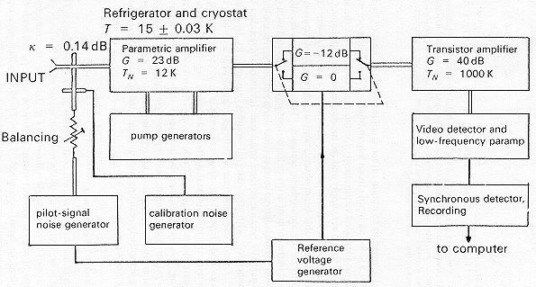
Figure 3. 1 A structural diagram of the 7.6-cm cooled radiometer. The radiometer was built along the lines of a noise-adding receiver design.
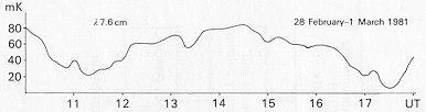
front end allowed us to obtain rather small losses at the input (0.14 dB, or Tfe = 9.5 K for an input circuit length of about 2 m). The price paid for this was: increased requirements for thermal stability and the stabilization of the power supply and the machinery in the radiometer, as well as limitations intrinsic to the noise-added receiver design: the impossibility of double-beam observations and the resultant removal of fluctuations in the atmospheric emission. These limitations manifest themselves in the form of drifts in the output signal associated with the weather and various internal sources which have not yet been completely studied, partially because of their small size. It can be shown that the drifts associated with the internal sources amount to less than 0.1 K h-1. One of the night-time recordings in good weather where the sky background (from the atmosphere and Galaxy; see Section 7) is mixed in with the instrumental drifts is shown in Fig. 3.2. The root-mean-square fluctuation s = 20mK on this record, which is many hours long; this indicates that the long-term stability of the receiver system is rather high. We are working on these limitations and other additional engineering measures for reducing the noise in the front end and more completely realizing the full potential of a cooled extremely low noise amplifier.
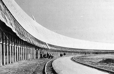
3.4. "Cooling" the Antenna
The antenna makes a significant contribution to the system noise. The measured noise temperature of the northern sector of the RATAN-600 as a function of elevation angle is shown in Fig. 3.3. Over the commonly used range of angles, without special anti-noise screens, but with the primary feed (a horn) optimized, Ta,n= 23–30K, which was considered to be perfectly satisfactory and did not noticeably decrease the
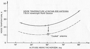
Figure 3.3 The antenna noise temperature of the north sector of the RATAN-600 as a function of altitude above the horizon. The asterisk indicates the antenna noise temperature in Experiment Cold, when the antenna was "cooled" using anti-noise screens (see the text and Fig. 3.5).
sensitivity of the first generation radiometers (Tsys
= 100 – 150 K). However, when using a very low-noise receiver system, such
antenna noise becomes completely unacceptable. The amount of noise from
the antenna is determined by spillover (illumination by radiation from
the ground through the error pattern of the mirrors). An experimental search
for the sources of this noise (Korol'kov, Maiorova, and Stotskii, 1978)
showed that the main source of noise is the regions above and below the
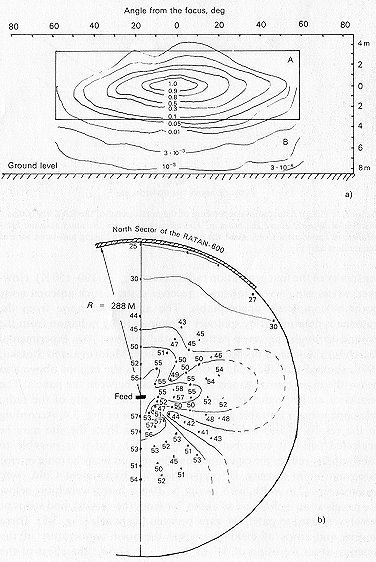
main mirror panels and the cracks between the panels. The results of an
inspection of the main mirror and the site of the radio telescope using
a portable generator are shown in Fig. 3.4. According to the results of
this inspection, the emission from the site may be neglected (since it
contributes less than 1 K), and it is possible to substantially reduce
the emission from the regions near the main mirror using anti-noise screens.
In preparation for Experiment Cold, wire mesh screens (2 m width, with
10 mm x 10 mm holes) were hung below the panels at an inclination of about
20o from the vertical, and strips of metal were used to patch
the gaps between the panels (Fig. 3.5). These screens and strips of metal
decreased the noise temperature of the antenna at an elevation of 51o
to Tnoise, ant = 11.5 K; the eOect of the wire mesh was
9 K, and the metal strips over the cracks between the panels yielded another
4 K. If the fact that the brightness temperature of the skj at 7:6 cm is
approximately 5.5 K (the 2.7 K cosmic background and 2.5 – 3 K of atmospheric
emission) is taken into account, the
excess noise temperature of the antenna due to the remaining scattering
is 6 K. The fact that the noise temperature of the antenna is so low indicates
that the RATAN-600 is rather well isolated from ground radiation, despite
the apparent "openness' of the periscopic system. By using relatively simple
screening techniques, it was possible to reduce the noise temperature of
the RATAN to values which are comparable to the Tnoise, ant
of the best low-noise antennas.
3.5. Calibration of the Radiometer in Terms of Antenna Temperature
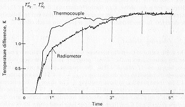
Measurements of the brightness temperatures of extended objects are extremely important in many observing programs; because of this, the absolute calibration of the radiometer in terms of brightness temperature is extremely important. As we said above, a calibration noise signal Tcal, from a noise generator (NG) is introduced into the front end of the receiver through a directional coupler (see the diagram in Fig. 3.1) to calibrate the observations while they are in progress. The absolute size of this calibration step was determined at the beginning of a cycle of observations using a matched cold load (cooled by liquid nitrogen) attached in place of the primary feed horn. A low thermal inertia cold load consisting of a cross (which was specially made from microwave absorber and mounted in a circular waveguide) was used for this. The nitrogen is poured directly into the waveguide, and the calibration temperature difference is obtained by measuring the boiling point of the nitrogen as the pressure changes in the cold load cryostat. The boiling point of nitrogen depends on the pressure in the following way:
We use an increase in pressure (obtained by partially closing an adjustable valve) to easily obtain a step
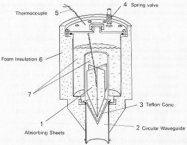
Figure 3.6 The low-inertia cold load (cooled by liquid nitrogen) inside the circular aveguide; the liquid nitrogen is poured into the waveguide (which contains a cross made 'absorber) and the surrounding volume. (I) Sheets of absorber; (2) circular waveguide; ) conical Teflon bafle; (4) valve; (5) thermocouple; (6) thermal insulation; (7) liquid nitrogen.
extremely low thermal inertia; on the portion of the curve where the
temperature is stable, the measurement accuracy is estimated to be ![]() 3%.
3%.
3.6. Total Noise Temperature and Sensitivity of the System
The ratio telescope – radiometer system (as it operated in Experiment
Cold) consisted of the following components, whose noise temperatures were
individually measured:
| antenna
front end paramp cryoblock contribution of thermal cascades (from the transistor amplifiers) |
Tnoise, ant =11.5 K (10 K)
Tfe =9.5 K (6 K) Tpa = 1.3 K (10 K) Tamp=5.0 K (0 K) ______________ Tsys= 37.3 K (26 K) |
This value of the root-mean-square fluctuation agrees with the system temperature given above. Can further substantial decreases in Tsys be expected? Unfortunately, a decrease of 30% is all that can realistically be expected; further reductions would require too much eftort.
3.7. Observing Method
The north sector of the radio telescope was used in the stationary mode
for the observations in the "Cold" program. In the first cycle (which was
begun on 17 March 1980), the antenna pattern was pointed towards the meridian
at a declination d1950=+4o54'
(an elevation of 51o) for three months, without resetting it.
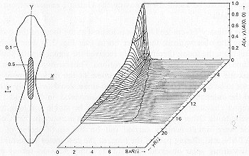
The shape of the antenna pattern of the sector is shown in Fig. 3.8 (Korzhavin,
1977). Because of the Earth's rotation, the radio telescope recorded the
emission at the main wavelength (7.6 cm) from a 24-hour long band of sky
10' in width with a reso.lution of 1' in hour angle; the solid angle of
the region surveyed was approximately 0.02 sr. In addition to 7.6 cm, work
was
also carried out at 1.35, 2.08, 3.9, 8.2, and 31 cm, using less sensitive receivers (see Table III.I). In addition to several independent astrophysical problems which were solved at these wavelengths, they were also used in support of the observations at the main wavelength of 7.6 cm:
|
|
|
|
|
|
|
|
|
|
The primary 7.6-cm feed horn was located at the focus of the system during the observations; the other horns (see Fig. 2.7) were slightly oftset from the focus; therefore, they received the signal slightly shifted in time (by up to 1m ) with slight aberrations. The transit mode (with the telescope stationary over the entire course of the cycle) allowed the sector to be equipped with temporary anti-noise shields relatively easily, and the antenna noise to be significantly decreased; in this mode, the antenna characteristics were guaranteed to be stable for long-term observations. Other observational programs not included in the "Cold" cycle were simultaneously carried out on the south sector of the RATAN, and, during part of the time, at the east sector (spectral line observations, solar observations, and the completely-sky-survey programs). The data were recorded on magnetic tape at a central recording point in the laboratory building, but, to insure reliability, a local backup data recording system (which later become the main system) based on an Elektronika-60 computer was installed at feed No. l.