|
|
|
|
|
4. Limiting Factors and Characteristics of the RATAN
4.1. Theoretical Sensitivity of the Radio Telescope and the Problem of Attaining it in Practice
The 7.6-cm radiometer described above definitely has very good characteristics; the amplifier itself has a noise temperature of approximately 10 K and a bandwidth of 500 MHz. Therefore, the problem of actually obtaining these characteristics in practice was particularly acute. The problem was divided into the "internal" (or engineering) problem of achieving the highest possible sensitivity (lowest possible noise); the problem of actually obtaining this sensitivity from the radio telescope-radiometer system with short integration times; and, finally, the problem of obtaining the maximum possible sensitivity in the essentially unknown field of studying extended regions of the sky at surface brightness levels of 1 mK or flux densities of 1 m Jy.*
In Experiment Cold, we dealt with all of these problems. We shall now list the limiting factors:
for an effective collecting area of 1000 m2. A further reduction in DTa and DPmin is possible, in principle, if the integration time is increased. These are the kinds of numbers we should aim for.
However, the actual state of affairs is not determined by Eqn (4.1) but by the sum
4.2.3 Atmosphere
The clearest example of the type of interference discussed above is
the emission from the atmosphere. With an average atmospheric emission
temperature of approximately 2.5 K at 7.6 cm (about 10% of the total
system temperature), the dispersion in the atmospheric interference (defined
as the root-mean-square deviation from the average over a time interval
of 1 hr) in all of the Cold experiments was a factor of 100 greater than
the theoretical radiometer sensitivity (averaged over two months of observations).
As is well known (Esepkina et al., 1973; Kaidanovskii et al.,
1982), when observing sources of small angular diameter (on the order
of a few beamwidths in size), an effective filtering method is widely used
– double-beam observations (in which the antenna records the difference
in the emission from two adjacent directions – source and background).
In our case, the observations were, by necessity, carried out using a single
beam and, because of this, other filtering methods were necessary. Two
methods seemed promising:
suppressing the low-frequency fluctuations during the data reduction, and using the correlation between the atmospheric emission at various wavelengths for cleaning. Let us briefly explain these two methods. At Pulkov and the RATAN, a fair amount of experience has been accumulated in studying the fluctuations in the atmospheric emission and suppressing them; this experience has been reviewed by Kaidanovskii et al. (1982). Two important conclusions follow from the measurements of the fluctuations in the emission from a cloudy atmosphere* that have been carried out at the RATAN over the last few years:
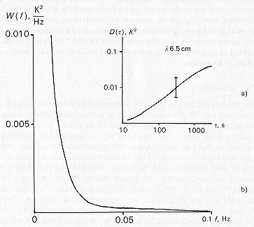
Figure 4.1 (a) An example of the structure function observed
at the RATAN-600 for the fluctuations in the radio emission from a cloudy
atmosphere. (b) The spectrum of the fluctuations in the atmospheric radio
emission corresponding to structure function (a).
(2) The fluctuations in the atmospheric emission at different wavelengths are correlated, and the correlation coefficient is very large. This property was first observed at the RATAN by Korol'kov and
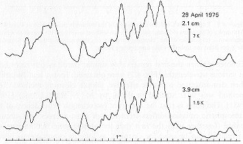
Figure 4.2 The radio emission from clouds at 2.1
and 3.9 cm (from observations at the RATAN-600 with the antenna stationary).
The correlation of the emission at these two wavelengths is very striking;
the intensity of the emission is proportional to l
-24
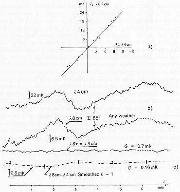
Figure 4.3 Experiment Cold: (a) correlation of the atmospheric emission at 4 and 8 cm; (A) samples of the scans (65 scans were averaged without selecting with respect to weather conditions); (c) samples of the "cleaning" process, i.e., subtraction of the 4-cm Scan from the 8-cm Scan multiplied by the appropriate factor.
Timofeeva when the first remarkably similar simultaneous recordings at various wavelengths (Fig. 4.2) were obtained; Ipatov and Bulaenko then demonstrated a rather effective, simple cleaning method. This method was later studied in detail by M. N. Kaidanovskii (1980, 1981). The point is that the spectrum (wavelength dependence) of the atmospheric emission differs from that of most sources; this circumstance (together with the fact that the atmospheric fluctuations are correlated) can be used for cleaning, as long as simultaneous observations are made at several different frequencies. In the cycle of Experiment Cold discussed here, observations were made at wavelengths of 1.35, 2, 3.9, 7.6 (the main wavelength), 8.2, and 31 cm. The observations at the shorter wavelengths (2 and 3.9cm; see Fig. 4.3) were used to remove the effects of the atmosphere from the images at 7.6 cm. When testing the correlation method (Kaidanovskii, 1981), we succeeded in suppressing the fluctuations in the atmospheric emission by approximately a factor of 10 (or somewhat more).*
Vitkovskii has proposed an interesting, simple method of dealing with strong atmospheric interference:
Suppose we have several scans of the same piece of sky which are of various quality (more precisely, with different contributions from atmospheric noise). The best of these scans (assume that it is the first) is then adopted as a reference for which the contribution from atmospheric noise can be neglected to first approximation. Then, all of the remaining records can be made so that they are no worse than the reference scan. In fact, subtracting the first record from the second, we remove the emission from sources, the Galaxy, and the Universe, and the remainder gives.us the contribution of the atmosphere to the second scan (since the contribution to the first is assumed to be zero), and so forth. These atmospheric components can be subtracted from all the records. This method was tested on 22 scans of the section 13h < a < 14h of Cold-1. This is successful provided
4.3. Confusion Noise
The noise-like fluctuations which arise as the antenna pattern moves over a sky filled with faint background sources is called "confusion noise". If the distribution of such sources over the sky is random, the
power at the output of the radio telescope will also vary in a random fashion. These fluctuations are not removed by long integration times, and they are diferent for diferent radio telescopes. If the "number of sources – flux density" curve (logN–logP, see Fig. 6.5) is known accurately, it is possible to estimate the confusion noise. In order to do this, however, it is necessary to know the shape as well as the eftecive solid angle of the antenna pattern of the radio telescope. This is essential when comparing the RATAN-600 to paraboloids. For the RATAN, the confusion noise becomes progressively smaller (according to the variation in the excess resolution coefficient h (see Section 4.6 for a discussion of the coefficient h)) as each of the following observing modes is used:
In more complex cases, Scheuer suggests the following relationship:
where P1 is the flux density at which the surface
density of sources is one radio source per antenna beam. However, if we
are interested in sufficiently large regions of the sky, it is possible
for high-resolution instruments to overcome confusion noise. We shall discuss
this in more detail in the following section.
4.4. Elimination of Discrete Sources
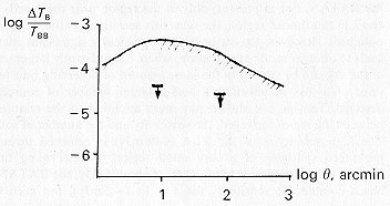
Usually, "specialization" of radio telescopes calls for a certain division of labor: aperture synthesis instruments study the discrete sources, while small antennas (including horns and dipoles) study the background emission. However, if the requirements on the accuracy with which the background emissioon is measured are increased, the background from faint (and bright!) radio sources inevitably becomes a limitation for low-resolution telescopes. If the contributions from such radio sources are not taken into account when observing, then, using the log N – log P curve (for a given wavelength), it is possible to find the limitations on the accuracy with which the surface brightness of extended features can be measured. The calculations carried out by Daneze et al. (1982) using the latest log N – log P data are shown in Fig. 4.4. The RATAN-600 allows the contributions from interfering sources to be taken into account to first order, down to a level of at least a few millijanskys (in Experiment Cold), i.e., the beam size of the radio telescope is much smaller than the region of background emission being studied. Essentially, the confusion noise can be reduced by at least a factor of 10 on scales of ~10'. See Fig. 6.4 for an illustration of the procedure by which sources were removed using Gaussian analysis. The next step in taking sources into account more carefully consists of complex studies of the same region using aperture synthesis instruments (the discrete sources) and the RATAN-600 (the background with the sources subtracted out); at present, the inability of aperture synthesis instruments to study large regions of the sky is the limitation here. Discussions are currently under way to organize observations of this type in a collaboration between the RATAN and the VLA.
4.5 Sky Surveys Using the RATAN-600
Carrying out surveys of the sky is one of the fundamental branches of astronomy. Without such surveys, our picture of the Universe is incomplete. The catalogs compiled when carrying out a sky survey are the basis for detailed studies by any of the methods available to humanity. The ideal survey would cover the entire sky at the highest sensitivity (and resolution!) available with current radio telescopes. But, since radio astronomers have not been able to develop a radio telescope for an experiment of this type, it is necessary to restrict ourselves to "specialized" surveys: to carry out either a rapid (rough) survey of the entire sky (paraboloids), or extremely deep surveys of very small sections of the sky (VLA). It is clear that the higher the desired sensitivity of the survey, the more difficult it is to survey a large section of the sky. Therefore, the extremely deep VLA surveys have little statistical significance (Keller-man, 1982), and the so-called rapid, "complete" surveys with para-boloids contain only the very strong sources, of which there are, once again, very few (see Kellerman, 1974).
The RATAN-600 occupies an intermediate position with respect to surveys. It is the only radio telescope at which a study of the entire sky with a resolution of 15" – 1' at wavelengths of 2, 3.5, and 8 cm, and a sensitivity higher than that of the so-called "strong-source surveys" is currently being carried out.
At its most sensitive wavelength, the VLA can make a map of a 1' x 1' region of the sky with an RMS noise level of approximately 0.08 mJy in 8 hr of synthesis. True, 8-hr exposures are also possible at the RATAN, but at present, only in the region near the North Pole. Here, in this limited region, the same flux sensitivity as the VLA can be obtained. However, the struggle for statistically significant material leads to another mode of operation, where a significantly larger section of the sky can be studied in the same amount of observing time (at the price of a loss in sensitivity), and a larger number of sources are detected. That is, one should pay more attention to the relationship between the region surveyed, the sensitivity and the number of sources. The high sensitivity of the VLA (0.08mJy) is achieved through a prolonged synthesis of a very small region. Transforming this to t = 1 s, this corresponds to an RMS of about 1 may; the RATAN-600 has a comparable sensitivity for t=1s (~ 5mJy), but even when observing with only one sector, the emission (integrated) from a 1' x 10' region (for observations using the plane periscopic refector on the south sector, a 1' x 40' region) is recorded. Because of this, a region which is a factor of 105 larger than at the VLA is surveyed in the course of 8 hrs of observations. It is possible to develop a way of carrying out such a survey in which the number of sources observed is as large as possible. Observations near the equator using the periscopic reflector of the RATAN (with a broad field of view in the vertical direction – approximately 40') turned out to be almost ideal from this point of view. In this mode, the RATAN-600, together with the high-sensitivity radiometer described in the previous section, has a record-breaking productivity – several hundred radio sources per day, which is approximately equal to the total number of radio sources which have been observed to date in all centimeter-wavelength surveys.
Thus, we see that there are two methods of increasing the number of
sources: increasing the depth to which a small fixed region of the sky
is surveyed (increasing the exposure), and actually increasing the area
surveyed. It is easy to show that where the log N – log P curve
is steep, the former is more efficient, while for extremely faint surveys,
where the slope of the log N – log P curve is small, the
latter is considerably more efficient. This method is widely used at the
RATAN-600, and this method was chosen as the basic method for Experiment
Cold in particular.
4.6. Brightness Temperature Sensitivity
If a radio telescope is attached to a matched load, the source and telescope are in thermodynamic equilibrium: all of the power received by the radio telescope from a distant object of arbitrary shape is reradiated back into space by the radio telescope. If we received radiation from the cosmos from an isotropic background with a temperature of 2.7 K over an angle of 4p sr, the so-called "effective antenna temperature" of the load resistance would be exactly equal to the brightness temperature of the background, i.e., 2.7 K. When studying an object of finite extent, it is necessary to know the shape of the source as well as the complete antenna pattern, i.e. the intensity of the radiation emitted by the radio telescope in all directions (over 4p sr). Only in this case is it possible to calculate the coefficient for the transformation between brightness temperature and antenna temperature. This calculation is based on thermodynamic arguments, since it is necessary to find out how much of the radiation emitted by the radio telescope will not be emitted toward the source of the radio emission. We shall take these losses into account using the two coefficients h1, and h2 , where h1, involves the losses in the antenna system (spillover and scattering from errors in the surface), and h2, takes the ratio of the solid angles (and the shapes) of the source and antenna pattern into account. Thus, we write the relationship between the brightness temperatures and antenna temperature as
where
| losses due to secondary mirror spillover:
losses due to main mirror spillover: losses due to the gaps between the panels: losses due to extended scattering (for an RMS surface error of 0.5 mm): |
0.97
0.80 0.965 0.994 |
It will be remembered that the aperture efficiency should not be confused with the coefficient h1, (as was done by Partridge (1980)). Moreover, if the errors in the surface are small, in order to make the beam efficiency approach unity, it is a good idea to decrease the aperture efficiency by decreasing the so-called aperture coefficient, i.e., underilluminating the main mirror. In fact this procedure was carried out in Experiment Cold by "refocusing" the system so that the secondary mirror illuminated a smaller portion of the main mirror than in the normal operating mode. As we have already mentioned, in Experiment Cold, the primary feedhorn was moved away from the focus in such a way that the secondary mirror formed a converging wave with the focus at the main mirror, rather than a plane wave. This led to a small RMS phase error over the aperture, but reduced the losses due to spillover (and decreased the antenna noise).
We shall now attempt to take the relative sizes of the telescope beam and the scales on which we are studying the variations in the 3-degree background into account, i.e., determine the coefficient h2,. For scales comparable to the size of the horizon at the hydrogen recombination epoch (several degrees), there is no correction: the entire antenna pattern (as well as the error pattern), which lies within the envelope of the pattern of a single element, is contained in a single inhomogeneity, and only the losses which were discussed above need to be taken into account. The situation is completely different when the antenna pattern is comparable to the size of the inhomogeneities being studied. This case is illustrated for a single inhomogeneity in Figs. 4.5(a – c). The relationship between the antenna temperature and the brightness temperature for each of these three cases is given by
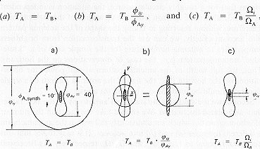
Figure 4.5 The relationship between the antenna temperature and brightness temperature for various ratios of the source size and beam size.
where WA is the effective solid angle of the antenna pattern within the pattern of a single element of the antenna. Here, we neglect all of the coefficients discussed above, but the values of h2, are
respectively. These relations are obvious from the same thermodynamic considerations discussed above. Two points still need to be clarified:
First, the quantity fAy ,. is not the vertical half-power beamwidth of the actual pattern. The antenna pattern of the RATAN-600 is a function of the elevation at which one is observing. For observations on the horizon, the "aperture" (i.e., as in the shape of the main reflecting surface of the RATAN-600 as it appears to an observer looking from the source) is a rectangle, and both cross-sections through the antenna beam (in azimuth as well as elevation) are Gaussian in form. For observations at intermediate elevations (our case), the aperture is shaped like a curved slit. In this case, the size of the center of the antenna pattern remains almost unchanged in azimuth but becomes much narrower in elevation (see Figs. 4.5 and 3.8). If the width of the antenna pattern is approximately fAy = 40' when observing on the horizon, then at the altitude of SS433 (at culmination), the size of the center of the beam in elevation is approximately 10'. However the narrowing of the antenna pattern in elevation occurs through the redistribution of energy over concentric surrounding regions centered on the axis of the antenna pattern. This means that for a roughly circular source, the situation is independent of altitude above the horizon from the viewpoint of thermodynamics. Therefore, without resorting to taking the shape of the antenna pattern into account exactly, we can use the transformation from brightness temperature to antenna temperature for the simple case of a "knife-edge" antenna pattern (i.e., the case of observations on the horizon). Thus, the full width of the antenna pattern at half-power for observations on the horizon (i.e., the size of the antenna pattern of a single element) should be used for fAy in case (b) above.Second, we are studying the statistical anisotropy of the sky, rather than an isolated fluctuation. We should take the fact that the number of inhomogeneities which simultaneously fall within the antenna beam is diferent for cases (a) and (b) into account. It is easy to see that this number n is equal to 1, fiy/fAy and Wi/WA respectively. As Bracewell and Conklin showed, taking the number of fluctuations per antenna beam into account leads to the following relationships between theantenna temperature and brightness temperature for cases (a), (b), and (c), respectively:
Thus, we must use the following relationships when reducing our data:
(b) in the search for protoclusters (scales of order fAy, synth, Fig. 4.5),
(c) when extrapolating the observational results to the scales of protogalaxies, globular clusters, and protostars (see Section 8),
where D2 synth is the synthesized aperture, and Wsynth is the solid angle of the synthesized beam, and Seff is the effective collecting area. In large synthesis systems, the coefficient h2 very small, on the order 10-6 for the VLA and 10-10 for VLBI; therefore, these systems have very low brightness temperature sensitivity. For the RATAN, the coefficient h2 , can also be used to characterize the excess resolution obtained in elevation because of the fact that the aperture appears to be curved when observing sources at elevations other than zero (the horizon), as was mentioned above; the value of h2 , can be determined using Eqn (4.8) and Fig. 3.5;
4.7. Conclusion: The Role of the RA TAN in Modern Radio Astronomy
As became clear in the 1970's, radio astronomers were incapable of building a completely universal instrument whose capabilities exceeded those of any other specialized radio telescope intended for solving a particular astrophysical problem. This can not be overcome by increasing the amount of money spent – both existing radio telescopes costing 100 million dollars and all of the enormous proposed telescopes costing tens of billions of dollars (such as, for example, the Cyclops project) suffer from this limitation.
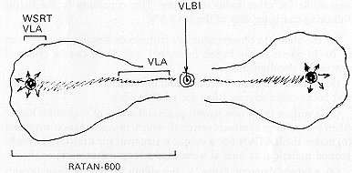
Modern radio telescopes have become specialized not only with respect to wavelength region or field of radio astronomy, but even with respect to a model of a typical radio galaxy (see Fig. 4.6). The giant "global" radio telescope networks only see the nuclear sources, which have sizes of ~ 10-3 arsec and a surface brightness very close to the limit, ~ 1012 K. They do not detect any of the main body of a radio galaxy (or, perhaps, they may see nothing at all, if the nucleus of the galaxy is not in an active phase. Moreover, they do not see any other objects – nebulae, H II regions, supernova remnants, main-sequence stars, the Sun, Moon, the planets and their statellites, etc.
The very large VLA-type aperture synthesis instruments only see the integrated emission from the nuclear source and the narrow streams and jets coming out of it, as well as the so-called "hot spots" in the radio components. The extended regions which emit most of the energy are only partially detected, and are sometimes completely invisible. Even the brightest source in the sky, Cas A, all of 4' in size, is completely invisible at the highest resolution of the VLA.
The RATAN-600 can detect the point source in a galaxy nucleus (but only from its integrated emission!) and obtain coarse images of the main body of a radio galaxy, but images of the nuclear source, jets, and hot spots are beyond its reach.
The largest paraboloids in the world are, as a rule, completely incapable of studying the structure of a typical radio galaxy, but they measure the integrated characteristics of radio galaxies very well, and are indispensible for studying the Galaxy, etc. It should be remembered that the bulk of the information on radio source statistics has been obtained using paraboloids at centimeter wavelengths. The fatal characteristic of a completely universal radio telescope is the same as for a person: a generalist knows a little bit about everything, in contrast to a narrow specialist, who knows everything within a very small field. In modern radio astronomy, as in modern society, the era of the Humboldts and Lomonosovs has come to an end. Progress in radio astronomy now occurs through the results obtained using specialized instruments.
In many respects, the RATAN-600 occupies an intermediate position between the large aperture-synthesis systems and the ordinary para-boloids. However, experience has shown that it is difterent from all other radio telescopes in some combinations of parameters; this allows us to use the RATAN-600 for problems which are practically impossible for other radio telescopes. This capability is due to the following characteristics of the RATAN:
In the first case, data is collected from a 1' x 1' (10-5
sr) region in 24 hr, but at high sensitivity. In the second case, the 24-hr
field of view is 2p rad x 1' ![]() 2 x 10⁻³ sr, with a sensitivity similar to that of the RATAN-600
in sky-survey mode. However, in this mode, the RATAN-600 observes a region
2p radian x 40' = 0.8 x 10⁻¹sr in
a 24-hr period, i.e., forty times larger. Therefore, specialization of
instruments makes sense: it is efficient to carry out statistical work
(but not on objects which are too faint) at the RATAN-600 and extremely
deep studies of selected regions using the VLA.
2 x 10⁻³ sr, with a sensitivity similar to that of the RATAN-600
in sky-survey mode. However, in this mode, the RATAN-600 observes a region
2p radian x 40' = 0.8 x 10⁻¹sr in
a 24-hr period, i.e., forty times larger. Therefore, specialization of
instruments makes sense: it is efficient to carry out statistical work
(but not on objects which are too faint) at the RATAN-600 and extremely
deep studies of selected regions using the VLA.
In the next section, we shall describe how we selected the problems best suited to the capabilities of an almost ideal radiometer.